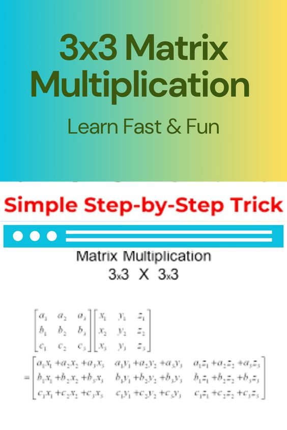
Matrix multiplication is a mathematical operation that takes two matrices and produces a third matrix.We will focus on understanding 3×3 matrix multiplication.
Understanding 3×3 Matrix Multiplication
Matrices are a powerful tool for representing and manipulating data. They can be used to represent a variety of things, such as transformations, relationships, and systems of equations.
Matrices and Their Dimensions
A matrix is a rectangular array of numbers. It is defined by its dimensions, which are the number of rows and columns. For example, a 3×3 matrix has 3 rows and 3 columns.
3×3 Matrices
A 3×3 matrix has 9 elements, which are arranged in a 3×3 grid. The elements of a matrix are usually denoted by a pair of subscripts, where the first subscript is the row number and the second subscript is the column number. For example, the element in the first row and second column of a 3×3 matrix is denoted by .
Using Matrices to Represent Transformations and Relationships
Matrices can be used to represent a variety of things, such as transformations, relationships, and systems of equations. For example, a 3×3 matrix can be used to represent a rotation in 3D space. The elements of the matrix represent the coefficients of the transformation, which are used to calculate the new coordinates of a point after it has been rotated.
Matrices can also be used to represent relationships between variables. For example, a 3×3 matrix can be used to represent a system of 3 equations with 3 unknowns. The elements of the matrix represent the coefficients of the equations, which are used to solve the system for the unknowns.
3×3 Matrix Multiplication
Matrix multiplication is the operation of multiplying two matrices together. The product of two matrices is a new matrix, which has the same number of rows as the first matrix and the same number of columns as the second matrix.
To multiply two matrices, we can use the following steps:
- Align the matrices so that the corresponding rows and columns are next to each other.
- For each row in the first matrix, multiply each element in the row by the corresponding element in the first column of the second matrix. Add the products together to get an element in the resulting product matrix.
- Repeat step 2 for each row in the first matrix.
The resulting product matrix will have the same number of rows as the first matrix and the same number of columns as the second matrix.
Step-by-Step Guide to 3×3 Matrix Multiplication
Matrix multiplication is a foundational operation in linear algebra with a myriad of applications across various fields. Understanding how to perform matrix multiplication accurately and efficiently is essential for both theoretical and practical purposes.
Setting Up Matrices for Multiplication
Matrix multiplication involves the multiplication of rows and columns to produce a new matrix. To get started, we need two matrices that satisfy specific conditions. Let’s introduce two 3×3 matrices, A and B:
Matrix A =
| a11 a12 a13 |
| a21 a22 a23 |
| a31 a32 a33 |
Matrix B =
| b11 b12 b13 |
| b21 b22 b23 |
| b31 b32 b33 |
It’s crucial to understand the concept of matching inner dimensions. The matrix A has dimensions m x n (3 rows and 3 columns), and matrix B has dimensions n x p (3 rows and 3 columns). The number of columns in matrix A must match the number of rows in matrix B for matrix multiplication to be valid.
Calculating Individual Entries
Matrix multiplication involves a systematic calculation of individual entries in the resulting matrix. Each entry in the resulting matrix is obtained by performing element-wise multiplication of the corresponding row in matrix A and the corresponding column in matrix B. The resulting products are then summed to yield the entry value.
For instance, let’s calculate the entry in the first row and first column of the resulting matrix C:
c11 = (a11 * b11) + (a12 * b21) + (a13 * b31)
Walkthrough Example: Calculating a Single Entry
To illustrate the process, let’s calculate the entry in the second row and third column of the resulting matrix C. Using the formula for matrix multiplication, we have:
c23
= (a21 * b13) + (a22 * b23) + (a23 * b33)
= (a21 * b13) + (a22 * b23) + (a23 * b33)
= (3 * 6) + (2 * 2) + (4 * 1)
= 18 + 4 + 4
= 26
Thus, the entry c23 in the resulting matrix C is 26.
Completing the Process: Systematic Calculation
Now that we’ve covered the calculation of individual entries, it’s time to complete the entire matrix multiplication process. This involves systematically calculating each entry in the resulting matrix C by pairing the rows of matrix A with the columns of matrix B and performing the element-wise multiplication and summation.
1. Begin with the first row of matrix A and the first column of matrix B. Calculate the entry in the first row and first column of matrix C using the element-wise multiplication and summation approach.
2. Move to the next column in matrix B and calculate the entry in the first row and second column of matrix C.
3. Continue this process for all columns in matrix B, resulting in the first row of matrix C.
4. Repeat steps 1 to 3 for the second and third rows of matrix A, calculating the remaining entries in matrix C.
Importance of Systematic Calculations
Systematic calculations are crucial when performing 3×3 matrix multiplication. A well-organized approach ensures that no entry is overlooked or miscalculated. The complexity of matrix multiplication makes it easy to make errors, and systematic calculations help mitigate this risk. By following a methodical process, you can maintain accuracy and confidence in your results.
Properties and Insights of 3×3 Matrix Multiplication
Matrix multiplication is a fundamental operation in linear algebra that underpins various applications across disciplines. As we delve deeper into the world of matrices, it becomes evident that matrix multiplication possesses intriguing properties that set it apart from other mathematical operations.
Non-Commutativity
Matrix multiplication, unlike addition, is non-commutative. This means that the order in which matrices are multiplied matters, and swapping the order often yields distinct results. To comprehend this property, it’s essential to understand the intricate interplay of transformations and combinations encapsulated within matrix multiplication.
Understanding the Non-Commutative Nature
Consider two 3×3 matrices, A and B:
A =
| a11 a12 a13 |
| a21 a22 a23 |
| a31 a32 a33 |
B =
| b11 b12 b13 |
| b21 b22 b23 |
| b31 b32 b33 |
Multiplying A by B results in matrix C:
C = A * B =
| c11 c12 c13 |
| c21 c22 c23 |
| c31 c32 c33 |
Reverse the order and multiply B by A to obtain matrix D:
D = B * A =
| d11 d12 d13 |
| d21 d22 d23 |
| d31 d32 d33 |
Visualizing the Difference: AB vs. BA
To grasp the concept more tangibly, consider a visual example. Imagine two matrices, A and B, representing 3D transformations. Matrix A could represent a rotation, and matrix B a scaling transformation. The order in which these transformations are applied indeed influences the outcome.
Suppose we apply transformation A followed by transformation B:
Result = B * A = AB
This sequence yields a transformed object with rotation followed by scaling.
Now, apply transformation B first, followed by transformation A:
Result = A * B = BA
In this case, the object undergoes scaling before rotation.
The key takeaway here is that the order of transformations directly impacts the final result. This non-commutative property echoes the intricate nature of matrix multiplication, reminding us that matrix operations involve intricate combinations of transformations that cannot be interchanged indiscriminately.
Associativity
Associativity is another intriguing property of matrix multiplication. This property grants us the freedom to group matrices and perform multiplication in various sequences while still yielding the same final result. This property may not be as immediately intuitive as non-commutativity, but it underlines the inherent elegance of matrix operations.
Unveiling the Associative Property
The associative property states that, when multiplying three or more matrices, the way they’re grouped doesn’t affect the final result. This means that matrices can be multiplied in any order, and as long as the correct pairings are maintained, the outcome remains consistent.
Let’s illustrate this property using three matrices, A, B, and C, and explore how their grouping impacts the result.
A =
| a11 a12 a13 |
| a21 a22 a23 |
| a31 a32 a33 |
B =
| b11 b12 b13 |
| b21 b22 b23 |
| b31 b32 b33 |
C =
| c11 c12 c13 |
| c21 c22 c23 |
| c31 c32 c33 |
Consider two different ways to multiply these matrices:
Scenario 1: (AB)C
First, we multiply matrices A and B to get matrix AB. Then, we multiply AB by matrix C.
(AB)C =
| a11b11 + a12b21 + a13b31 a11b12 + a12b22 + a13b32 a11b13 + a12b23 + a13b33 |
| a21b11 + a22b21 + a23b31 a21b12 + a22b22 + a23b32 a21b13 + a22b23 + a23b33 |
| a31b11 + a32b21 + a33b31 a31b12 + a32b22 + a33b32 a31b13 + a32b23 + a33b33 |
Scenario 2: A(BC)
Next, multiply matrices B and C to get matrix BC. Then, multiply matrix A by BC.
A(BC) =
| a11(b11c11 + b12c21 + b13c31) + a12(b11c12 + b12c22 + b13c32) + a13(b11c13 + b12c23 + b13c33) |
| a21(b21c11 + b22c21 + b23c31) + a22(b21c12 + b22c22 + b23c32) + a23(b21c13 + b22c23 + b23c33) |
| a31(b31c11 + b32c21 + b33c31) + a32(b31c12 + b32c22 + b33c32) + a33(b31c13 + b32c23 + b33c33) |
Maintaining Equivalence
The remarkable insight here is that despite the differing arrangements, (AB)C and A(BC) result in identical matrices. This highlights the flexibility of grouping in matrix multiplication, making it a powerful and versatile operation.
Understanding the Significance
Non-commutativity and associativity reveal profound aspects of matrix multiplication. The non-commutative nature reminds us of the intricacies inherent in transforming one mathematical entity into another. The associative property showcases the elegance of matrix operations, allowing us to manipulate groupings without altering the final outcome. Together, these properties demonstrate the depth and complexity embedded within matrix multiplication, underscoring its significance in mathematics and applications across various fields.
Practice Problems of Mastering 3×3 Matrix Multiplication
To solidify your understanding of 3×3 matrix multiplication, it’s essential to engage with practice problems that challenge your skills and intuition. By working through these problems, you’ll gain confidence in applying the concepts discussed earlier and enhance your proficiency in matrix multiplication.
Problem 1: Matrix Product of A and B
Given matrices A and B, perform the matrix multiplication AB.
Matrix A=
| 3 1 2 |
| 0 2 4 |
| 1 3 5 |
Matrix B=
| 2 1 0 |
| 3 2 1 |
| 1 0 2 |
Solution 1: Matrix Product of A and B
Calculate the individual entries of the resulting matrix AB:
For the entry in the first row and first column:
3*2 + 1*3 + 2*1 = 6 + 3 + 2 = 11
For the entry in the first row and second column:
3*1 + 1*2 + 2*0 = 3 + 2 + 0 = 5
Continue this process to calculate all entries of the resulting matrix AB.
Resulting Matrix AB:
| 11 5 10 |
| 14 8 14 |
| 20 11 19 |
Problem 2: Exploring Non-Commutativity
Given matrices C and D, calculate both CD and DC. Comment on their results to illustrate non-commutativity.
Matrix C=
| 1 2 3 |
| 4 5 6 |
| 7 8 9 |
Matrix D=
| 9 8 7 |
| 6 5 4 |
| 3 2 1 |
Solution 2: Exploring Non-Commutativity
Calculate the matrix products CD and DC:
For the matrix product CD:
| 1*9+2*6+3*3 1*8+2*5+3*2 1*7+2*4+3*1 |
| 4*9+5*6+6*3 4*8+5*5+6*2 4*7+5*4+6*1 |
| 7*9+8*6+9*3 7*8+8*5+9*2 7*7+8*4+9*1 |
Perform the calculations and simplify each entry.
For the matrix product DC:
| 9*1+8*4+7*7 9*2+8*5+7*8 9*3+8*6+7*9 |
| 6*1+5*4+4*7 6*2+5*5+4*8 6*3+5*6+4*9 |
| 3*1+2*4+1*7 3*2+2*5+1*8 3*3+2*6+1*9 |
Perform the calculations and simplify each entry.
Now, compare the resulting matrices CD and DC. You’ll notice that they are not the same, demonstrating the non-commutative nature of matrix multiplication.
Problem 3: Transformation Matrix Application
Matrix E represents a 2D transformation. Matrix F defines the coordinates of a point in the original space. Calculate the transformed coordinates using matrix multiplication EF.
Matrix E=
| 2 -1 |
| 3 2 |
Matrix F=
| 5 |
| 7 |
Solution 3: Transformation Matrix Application
To calculate the transformed coordinates using matrix multiplication EF, perform the following calculations:
For the entry in the first row and first column:
2*5 + -1*7 = 10 – 7 = 3
For the entry in the second row and first column:
3*5 + 2*7 = 15 + 14 = 29
The transformed coordinates are:
| 3 |
| 29 |
Problem 4: Applying Associativity
Given matrices G, H, and I, calculate (GH)I and G(HI). Comment on the results to illustrate the property of associativity.
Matrix G=
| 2 1 3 |
| 0 4 1 |
| 5 2 6 |
Matrix H=
| 3 0 1 |
| 2 5 4 |
| 1 3 2 |
Matrix I=
| 6 1 2 |
| 4 3 5 |
| 0 7 8 |
Solution 4: Applying Associativity
Let’s calculate (GH)I and G(HI) to illustrate the property of associativity:
For (GH)I:
Calculate matrix GH first:
GH = G * H
Now, calculate (GH)I:
(GH)I = GH * I
Similarly, for G(HI):
Calculate matrix HI first:
HI = H * I
Now, calculate G(HI):
G(HI) = G * HI
Compare the results of (GH)I and G(HI). You’ll find that they are the same, demonstrating the property of associativity in matrix multiplication.
Problem 5: Applying Matrix Multiplication in Computer Graphics
Matrix J represents a scaling transformation, and matrix K defines the original coordinates of a point in 2D space. Calculate the coordinates of the scaled point using matrix multiplication JK.
Matrix J (Scaling Transformation):
| 3 0 |
| 0 2 |
Matrix K (Original Coordinates):
| 4 |
| 7 |
Solution 5: Applying Matrix Multiplication in Computer Graphics
To calculate the scaled coordinates using matrix multiplication JK, perform the following calculations:
For the entry in the first row and first column:
3*4 + 0*7 = 12 + 0 = 12
For the entry in the second row and first column:
0*4 + 2*7 = 0 + 14 = 14
The scaled coordinates are:
| 12 |
| 14 |
Problem 6: Real-World Applications of Matrix Multiplication
Consider two matrices L and M. Matrix L represents a system of linear equations, and matrix M contains variables. Solve for the variables using matrix multiplication.
Matrix L=
| 2 1 3 |
| 1 -1 2 |
| 3 2 -1 |
Matrix M (Variable Matrix):
| x |
| y |
| z |
Solution 6: Real-World Applications of Matrix Multiplication
To solve for the variables x, y, and z, we can set up the equation LM = N, where N is the result matrix:
Matrix N (Result Matrix):
| 6 |
| 3 |
| 10 |
We have the equation LM = N, which can be written as:
| 2 1 3 | | x | | 6 |
| 1 -1 2 | * | y | = | 3 |
| 3 2 -1 | | z | | 10 |
Solve for the variables using matrix multiplication and equation solving techniques. Once the values of x, y, and z are obtained, you have successfully applied matrix multiplication to solve a real-world problem involving a system of linear equations.
Problem 7: Multi-Step Transformation
Matrix P represents a translation, matrix Q defines a rotation, and matrix R represents a scaling. Given a point’s coordinates represented by matrix S, calculate the final transformed coordinates using matrix multiplication.
Matrix P (Translation):
| 1 0 2 |
| 0 1 3 |
| 0 0 1 |
Matrix Q (Rotation):
| 0 -1 0 |
| 1 0 0 |
| 0 0 1 |
Matrix R (Scaling):
| 2 0 0 |
| 0 3 0 |
| 0 0 1 |
Matrix S (Original Coordinates):
| 4 |
| 5 |
| 1 |
Solution 7: Multi-Step Transformation
To calculate the final transformed coordinates using matrix multiplication PQR, perform the following calculations:
1. Calculate the intermediate matrix PQ:
PQ = P * Q
2. Calculate the intermediate matrix PQR:
PQR = PQ * R
3. Apply the PQR transformation to matrix S:
Result = PQR * S
Perform the necessary matrix multiplications and calculations to obtain the final transformed coordinates.
Problem 8: Investigating Identity Matrix
Matrix I3 is the identity matrix of order 3. Calculate the matrix product of I3 with another arbitrary 3×3 matrix T.
Matrix I3 (Identity Matrix):
| 1 0 0 |
| 0 1 0 |
| 0 0 1 |
Matrix T (Arbitrary 3×3 Matrix):
| a b c |
| d e f |
| g h i |
Solution 8: Investigating Identity Matrix
To calculate the matrix product of I3 with matrix T, perform the multiplication as follows:
Result = I3 * T
| 1 0 0 | | a b c |
| 0 1 0 | * | d e f |
| 0 0 1 | | g h i |
The resulting matrix will be the same as matrix T:
| a b c |
| d e f |
| g h i |
This demonstrates an interesting property of the identity matrix: when it’s multiplied with any matrix, it leaves the matrix unchanged.
Problem 9: Matrix Multiplication in Cryptography
Matrix U represents an encryption key, and matrix V represents a message. Calculate the encrypted message using matrix multiplication UV.
Matrix U (Encryption Key):
| 3 1 |
| 2 4 |
Matrix V (Message):
| 10 |
| 5 |
Solution 9: Matrix Multiplication in Cryptography
To calculate the encrypted message using matrix multiplication UV, perform the following calculations:
For the entry in the first row and first column:
3*10 + 1*5 = 30 + 5 = 35
For the entry in the second row and first column:
2*10 + 4*5 = 20 + 20 = 40
The encrypted message is:
| 35 |
| 40 |
These encrypted values can be transmitted securely and decrypted using the inverse of matrix U.
Problem 10: Reflection Transformation
Matrix W represents a reflection transformation. Given a point’s coordinates represented by matrix X, calculate the coordinates of the reflected point using matrix multiplication WX.
Matrix W (Reflection):
| -1 0 |
| 0 1 |
Matrix X (Original Coordinates):
| 6 |
| 8 |
Solution 10: Reflection Transformation
To calculate the coordinates of the reflected point using matrix multiplication WX, perform the following calculations:
For the entry in the first row and first column:
-1*6 + 0*8 = -6 + 0 = -6
For the entry in the second row and first column:
0*6 + 1*8 = 0 + 8 = 8
The coordinates of the reflected point are:
| -6 |
| 8 |
These practice problems cover various aspects of 3×3 matrix multiplication, showcasing its relevance in diverse fields, from geometry to cryptography. By working through these problems and understanding the solutions, you’ll learn matrix multiplication and its applications fast.

3×3 Matrix Multiplication Learn math fast Cool math Playground art project